dPCR Data Analysis and Interpretation

The Universal dPCR Analysis Workflow

dPCR data analysis always follows four steps:

1. Signal detection: Fluorescence measurement (flow cytometry for droplets, imaging for chips).
2. Quality control: Check partitions, determine valid/invalid samples.
3. Threshold setting: Separate positive from negative partitions.
4. Statistical correction: Mathematical transformation of positive fraction to absolute concentration, normally using Poisson correction.

After dPCR amplification, each partition’s fluorescence intensity is measured. Data from the partitions tells us which samples are valid and which are not. Partitions exhibiting fluorescence above background are classified as positive (containing target DNA), while those at background levels are negative. This binary classification is the foundation of digital PCR's absolute quantification capability, but it can be challenging to know where to set the threshold for positive vs negative partitions.

The next step is calculating the initial target concentration. Because partitions may contain more than one target molecule, the simple ratio of positive to total partitions underestimates true concentration. The Poisson correction accounts for this by calculating the probability of zero molecules per partition based on the observed negative fraction.

Figure 1. The universal dPCR analysis workflow, with the four core steps: signal detection, quality control, threshold setting, and statistical correction.

System and manufacturer software or manual analysis

The most common dPCR data analysis software is from dPCR system manufacturers, such as Bio-Rad QuantaSoft, Qiagen QIAcuity Software Suite, or Roche LightCycler Software. These automate threshold setting, Poisson corrections, and quality flagging through guided graphical interfaces, providing quick analysis with minimal bioinformatics expertise.

These solutions integrate seamlessly with their respective hardware but offer limited customization for non-standard workflows. Alternatives include open-source R packages (e.g., ddpcr, dpcr) and Python libraries. These allow for manual gating, custom clustering algorithms, and batch processing of large datasets, providing the most flexibility for complex experimental designs or cross-platform comparisons. These alternatives demand a greater time investment and statistical knowledge, but offer better analytical control.

Wondering which applications benefit from dPCR? Check out our first article on dPCR applications such as liquid biopsy, CNV, and pathogen detection.

dPCR Quality Control, Partition Classification, And Threshold Setting

Once fluorescence has been analyzed, decisions must be made. Which samples need to be excluded because of poor data? Which partitions are positive, and which are negative? The choices made here can significantly alter the results of the experiment.

Quality control checkpoints

Before accepting the results from each sample and the whole experiment, verify four parameters:

1. Partition counts: Require >10,000 accepted partitions per well (or check specific system recommendations) for reliable Poisson statistics, exclude wells below this threshold.¹
2. Positive fraction: Target 5–80% positive partitions, as optimal precision occurs at ~20% negative (1.6 copies/partition).² Beware of samples with >95% positive partitions (saturation) or <1% positive partitions (insufficient signal), as they will have high relative uncertainty.
3. No-template controls (NTC) contamination: If these have positive partitions with similar fluorescence intensity levels as positive controls, the samples are likely contaminated.
4. Positive control validation: Measured copy numbers must fall within expected confidence intervals. If this is not the case, you can’t trust the rest of the experiment’s results.

If you have multiple replicates, you can discard individual outlier wells results. However, if your controls show abnormal results, you should repeat the entire experiment.

Binary classification and threshold setting

All dPCR samples require amplitude-based discrimination to classify partitions as positive or negative.

Ideally, positive samples have much higher fluorescence signals than negative samples. But sometimes the difference might not be so pronounced. Additionally, each fraction may span large variations of fluorescence intensity. You must decide from which fluorescence value each fraction (positive and negative) starts. This is the threshold.

Threshold setting optimization utilizes NTC amplitude distributions to set negative boundaries.³ Then, automated algorithms (density-based clustering for droplets, image analysis for chips) or manual gating assign ambiguous partitions to the nearest clusters.

Remember that validation requires visual confirmation that positive and negative populations exhibit >2 standard deviations separation to ensure results are unambiguous.

Nonetheless, there are common artifacts. The more prominent ones are “rain” and “stars”:⁴

1. Rain: partitions that are between the positive and the negative main clusters are called rain. These can be positive samples with probe degradation, amplification problems, or other challenges that result in lower fluorescence. Rain partitions can also be negative samples showing intermediate fluorescence intensity due to primer dimers, non-target amplification, or, in multiplexed samples, excitation of fluorophores detecting other targets.⁵
2. Stars: high-fluorescence partitions, above the positive fraction. These can be artifacts (clusters of probes, dust), and should not always be counted as positives. They could also come from target and non-target amplification taking place in the same partition.

Figure 2. dPCR plots showing positive fractions (blue clusters), and negative fractions (grey clusters). Between the main fractions, the rain phenomenon can be seen (circled in blue). Thresholds are represented by a pink line. In panel A, the threshold assigned most of the rain to the positive fraction, while in B, it assigned them to the negative fraction. Circled in red are two examples of stars. Modified from Figure 5 of The dMIQE Group and Huggett JF. Clin Chem. 2020;66(8):1012–1029.⁶

Statistics and Interpretation

The last thing to do is to correct the data to obtain the absolute number of copies. The most common way to calculate copies per microliter is to use the Poisson correction.⁷ However, other methods have gained some traction in the last few years. Lastly, additional considerations must be taken into account when analyzing multiplex dPCR data.

Absolute quantification using Poisson correction

Digital PCR’s power derives from binary endpoint detection: each partition scores as positive (1) or negative (0) after PCR, independent of amplification efficiency.

Molecules are assumed to distribute randomly among partitions, following Poisson statistics, so the fraction of negative partitions (p₀) directly relates to the average molecules per partition (λ). But if 8,000 partitions are positive out of 20,000, that does not mean there are 8,000 target molecules, as some partitions may have 2, 3, or more copies.

The fraction of negative partitions follows a Poisson distribution. The average molecules per partition (λ) is calculated as:

λ = −ln(p₀) or equivalently λ = −ln(1−p)

Where p₀ = fraction of negative partitions (negative partitions/ total partitions)

Total copies per reaction = λ × (total partitions)

Concentration = Total copies / reaction volume (in µL) = copies/µL

Example: If 8,000 of 20,000 partitions are positive (40% positive, 60% negative):

• λ = −ln(0.60) = 0.51 copies per partition
• Total copies = 0.51 × 20,000 = 10,200 copies<
• Concentration = 10,200 / 20 µL = 510 copies/µL

Statistical precision improves with more partitions: the coefficient of variation decreases with partition number, meaning 20,000 partitions yield ~0.7 % theoretical precision, while 10,000 partitions provide ~1 %.

95 % confidence intervals are calculated from the binomial distribution of positive/negative counts, widening as positive fractions approach saturation (>95 %) or scarcity (<1 %).

Unsure about how to set up a good experiment to obtain good confidence intervals? Our guide on dPCR assay design gives you practical tips to do so.

Alternative statistical methods

Standard dPCR quantification assumes random distribution of molecules (Poisson distribution) and identical partition volumes, but these assumptions can be violated (like partition volume differences, non‑random loading, etc.).⁸

When partition volumes vary, pure Poisson models become biased at higher concentrations, and extended models like Poisson-Plus have been developed to help with that.⁹ Other, more flexible approaches can provide higher accuracy in certain circumstances.

For uncertainty estimation, several papers explicitly model the number of positive partitions as binomial (or multinomial in multiplex) and develop methods (delta method, binomial bootstrap “BinomVar”, “NonPVar”, etc.) that work on the discrete positive/negative counts instead of assuming an ideal infinite‑partition Poisson process.¹⁰

In parallel, generalized linear (mixed) models with complementary log-log links have been proposed. These embed the Poisson model in a GLM framework, allowing partition volume to be included as an offset, and experimental factors (such as assay, replicate, or treatment) to entered as covariates. This improves variance estimates when additional error sources are present.¹¹

For routine applications where partitioning is approximately random and technical variability is limited, standard Poisson‑based quantification is generally adequate. However, if precise uncertainty quantification or method validation is required, other models provide more flexible (and often more accurate) variance estimates than simple Poisson formulas.

For standardized dPCR data analysis and reporting, follow the dMIQE 2020 guidelines, the accepted community standard for digital PCR experiment reporting.⁶

Multiplexing considerations

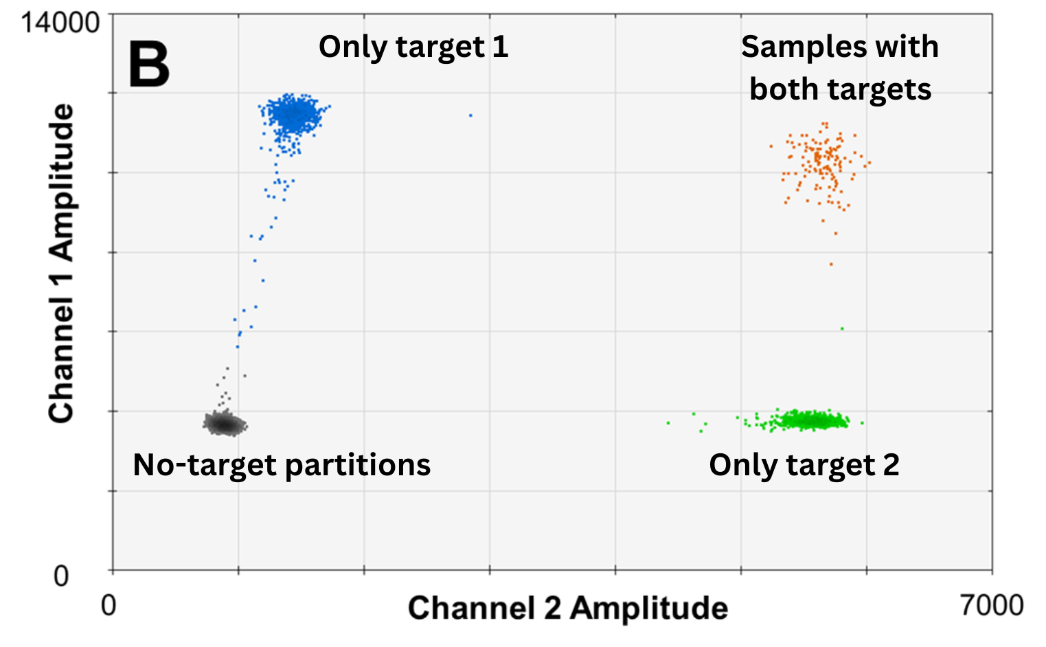
Figure 3. Example of output of multiplex dPCR with two targets. Dots represent partitions with none, one, or two targets. Note that the rain phenomenon is still visible. Modified from Hughesman CB, Lu XJD, et al. PLoS One. 2016;11(8):e0161274, Supplementary Figure 2 B.¹²

Multiplexed dPCR requires mathematical deconvolution to separate overlapping fluorescence signals. Spillover compensation matrices correct spectral bleed-through between channels, particularly critical in six- to seven-color systems.

The analysis involves solving linear equations where total fluorescence in each channel equals the sum of individual fluorophore contributions multiplied by their spectral overlap coefficients.¹³

Reference gene normalization in multiplex CNV assays requires propagation of uncertainty from both numerator and denominator, compounding confidence intervals.¹⁴

Remember to always validate multiplex performance by comparing single-plex versus multiplex results. Significant deviation indicates primer competition or probe cross-reactivity requiring assay redesign.

This article is part of a 3-part series on digital PCR. Continue reading:

• dPCR basics, dPCR vs qPCR, and when to use dPCR
• dPCR assay design and experiment planning
• Inside the Application Digital PCR (dPCR) Hub

Frequently Asked Questions (FAQs)

Q1: What is “rain” in dPCR? Rain in ddPCR refers to partitions with fluorescence levels between the positive and negative clusters. This is caused by partial amplification, probe degradation, or inhibitors, and rain partition assignment to either fraction directly affects your final count.

Q2: When should I use open-source tools like R instead of manufacturer software for dPCR analysis? Manufacturer software is sufficient for standard single-plex or low-plex workflows on their own hardware. Open-source tools become valuable when you need custom gating algorithms, cross-platform comparisons, batch processing of large datasets, or advanced statistical models, like Poisson-Plus or GLM-based methods. These go beyond what proprietary interfaces offer.

Q3: How does the Poisson correction change my results compared to a simple positive/total count? A simple ratio always underestimates true concentration because it ignores partitions containing more than one molecule. The Poisson correction determines the average number of target DNA molecules per partition. Multiply that by the total partitions, and you have the total quantity of target DNA molecules in your whole sample.

References

1. van Ginkel JH, Huibers MMH, et al. Droplet digital PCR for detection and quantification of circulating tumor DNA in plasma of head and neck cancer patients. BMC Cancer. 2017;17:428.https://doi.org/10.1186/s12885-017-3424-0

2. Majumdar N, Wessel T, et al. Digital PCR modeling for maximal sensitivity, dynamic range and measurement precision. PLoS One. 2015;10(3):e0118833.https://doi.org/10.1371/journal.pone.0118833

3. Kaisar MMM, Kristin H, et al. Optimization and application of digital droplet PCR for the detection of SARS-CoV-2 in saliva specimen using commercially available kit. Biol Methods Protoc. 2024;9(1):bpae068.https://doi.org/10.1093/biomethods/bpae068

4. Porco D, Hermant S, et al. Getting rid of ‘rain’ and ‘stars’: mitigating inhibition effects on ddPCR data analysis, the case study of the invasive crayfish Pacifastacus leniusculus in the streams of Luxembourg. PLoS One. 2022;17(11):e0275363.https://doi.org/10.1371/journal.pone.0275363

5. Lievens A, Jacchia S, et al. Measuring digital PCR quality: performance parameters and their optimization. PLoS One. 2016;11(5):e0153317.https://doi.org/10.1371/journal.pone.0153317

6. The dMIQE Group and Huggett JF. The Digital MIQE Guidelines Update: Minimum Information for Publication of Quantitative Digital PCR Experiments for 2020. Clin Chem. 2020;66(8):1012–1029. https://doi.org/10.1093/clinchem/hvaa125

7. Sedlak RH, Jerome KR. Viral diagnostics in the era of digital PCR. Diagn Microbiol Infect Dis. 2012;75(1):1–4.https://doi.org/10.1016/j.diagmicrobio.2012.10.009

8. Trypsteen W, Vynck M, et al. ddpcRquant: threshold determination for single channel droplet digital PCR experiments. Anal Bioanal Chem. 2015;407(19):5827–5834.https://doi.org/10.1007/s00216-015-8773-4

9. Majumdar N, Banerjee S, et al. Poisson plus quantification for digital PCR systems. Sci Rep. 2017;7:9617.https://doi.org/10.1038/s41598-017-09183-4

10. Chen Y, De Spiegelaere W, et al. Flexible methods for uncertainty estimation of digital PCR data. iScience. 2025;28(3):111772.https://doi.org/10.1016/j.isci.2025.111772

11. Vynck M, Vandesompele J, et al. Flexible analysis of digital PCR experiments using generalized linear mixed models. Biomol Detect Quantif. 2016;9:1–13.https://doi.org/10.1016/j.bdq.2016.06.001

12. Hughesman CB, Lu XJD, et al. A robust protocol for using multiplexed droplet digital PCR to quantify somatic copy number alterations in clinical tissue specimens. PLoS One. 2016;11(8):e0161274.https://doi.org/10.1371/journal.pone.0161274

13. Madic J, Zocevic A, et al. Three-color crystal digital PCR. Biomol Detect Quantif. 2016;10:34–46.https://doi.org/10.1016/j.bdq.2016.10.002

14. Yener D, Busby EJ, et al. Multiplexed digital PCR reference gene measurement for genomic and cell-free DNA analysis. Cells. 2025;14(19):1544.https://doi.org/10.3390/cells14191544